dismo tutorial¶

dismo is a pacakge that allows creation, simulation and analysis of discrete spatial models of complex non-regular shapes, like the ones depicted below

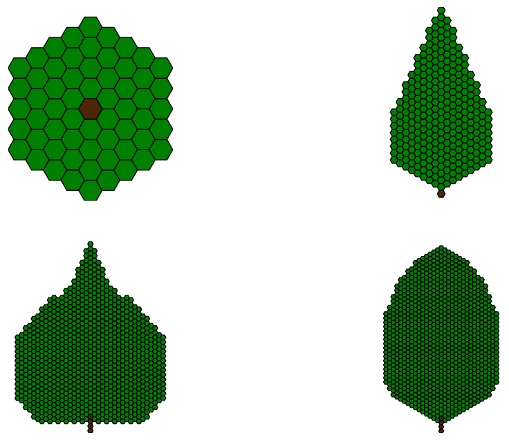
To allow you to quickly exchange the geometric representation of your problem, dismo separates the grid onto which cells are being placed and the actual model implementation.

Let's start by importing the usual scientific packages.

In [1]:

from __future__ import annotations

import math
from dataclasses import dataclass
from typing import Callable, Iterable, cast

import matplotlib.pyplot as plt
import numpy as np
import pandas as pd
from IPython.core.display import HTML
from matplotlib import animation
from matplotlib.animation import FuncAnimation
from matplotlib.axes import Axes
from matplotlib.figure import Figure
from numpy.typing import NDArray
from typing_extensions import override

from dismo import grids, models

Array = NDArray[np.float64]

from __future__ import annotations import math from dataclasses import dataclass from typing import Callable, Iterable, cast import matplotlib.pyplot as plt import numpy as np import pandas as pd from IPython.core.display import HTML from matplotlib import animation from matplotlib.animation import FuncAnimation from matplotlib.axes import Axes from matplotlib.figure import Figure from numpy.typing import NDArray from typing_extensions import override from dismo import grids, models Array = NDArray[np.float64]

Could not find cannot import name 'dopri5' from 'assimulo.lib' (/opt/conda/envs/py311/lib/python3.11/site-packages/assimulo/lib/__init__.py)
Could not find cannot import name 'rodas' from 'assimulo.lib' (/opt/conda/envs/py311/lib/python3.11/site-packages/assimulo/lib/__init__.py)
Could not find cannot import name 'odassl' from 'assimulo.lib' (/opt/conda/envs/py311/lib/python3.11/site-packages/assimulo/lib/__init__.py)
Could not find ODEPACK functions.
Could not find RADAR5
Could not find GLIMDA.

Grids¶

dismo features a number of pre-defined grids that should be sufficient for most use cases.
There are grids for one, two and three-dimensional coordinate systems.
In all cases neighbors are counted as the cells sharing a border, not just an single point.
However, it is straight-forward to define custom grids in which this behaviour is allowed.

1D¶

In the one-dimensional case we supply the RodGrid, in which all cells (except the border ones) have exactly two neighbors.

In [2]:

grid = grids.RodGrid((11,))
fig, ax = grid.plot_axes()
grid.plot_grid(ax=ax)
grid.plot_cell_coordinates(ax=ax, fontsize=11)

grid = grids.RodGrid((11,)) fig, ax = grid.plot_axes() grid.plot_grid(ax=ax) grid.plot_cell_coordinates(ax=ax, fontsize=11)

2D¶

For the two-dimensional case we supply a TriGrid, SquareGrid and HexGrid, which use triangular, cartesian or hexagonal coordinates and in which each cell (except the border ones) has three, four and six neighbors respectively.
dismo takes over calculating the respective neighbors for you, so you don't need to worry about this.

For those interested: the hexagonal coordinate system is Oddq.

In [3]:

for ax, grid_type in zip(
    plt.subplots(1, 3, figsize=(15, 5))[1],
    (grids.TriGrid, grids.SquareGrid, grids.HexGrid),
):
    grid = grid_type((5, 5))
    grid.plot_axes(ax=ax)
    grid.plot_grid(ax=ax)
    grid.plot_cell_coordinates(ax=ax, fontsize=11)

for ax, grid_type in zip( plt.subplots(1, 3, figsize=(15, 5))[1], (grids.TriGrid, grids.SquareGrid, grids.HexGrid), ): grid = grid_type((5, 5)) grid.plot_axes(ax=ax) grid.plot_grid(ax=ax) grid.plot_cell_coordinates(ax=ax, fontsize=11)

3D¶

For the three-dimensional case we supply the CubeGrid, in which each cell (except the border ones) has 6 neighbors.

In [4]:

grid = grids.CubeGrid((3, 3, 3))
fig, ax = grid.plot_axes()
grid.plot_grid(ax=ax)
grid.plot_cell_coordinates(ax=ax, fontsize=11)

grid = grids.CubeGrid((3, 3, 3)) fig, ax = grid.plot_axes() grid.plot_grid(ax=ax) grid.plot_cell_coordinates(ax=ax, fontsize=11)

In [ ]:

In [ ]:

In [ ]:

Plant leaf models¶

dismo was initially build to allow modelling discrete cells in a plant leaf.
There are three models that are pre-defined, which increasingly incoorporate more mechanisms:

• MesophyllModel contains
  • sucrose as the only system variable
  • a mesophyll celltype
  • a crude, saturating photosynthesis function with two parameters ps_vmax and ps_km
  • a diffusion function for sucrose between cells with one parameter suc_meso_to_meso
• VeinModel extends MesophyllModel by
  • a vein celltype
  • diffusion functions for vein-to-vein, as well as mesophyll-to-vein transport
  • a sucrose outflux function at the vein base
• StomataModel extends VeinModel by
  • a stomata celltype
  • CO2 as a second system variable
  • influx and transport processes for CO2

Mesophyll models¶

As all of that can be quite overwhelming, let's simplify.
We'll start with just the MesophyllModell and disable the photosynthesis function by setting the respective parameter to zero.
Then we'll set the initial conditions of one cell to one and will observe the diffusion process.

In [5]:

def make_mesophyll_rod_model() -> models.MesophyllModel:
    model = models.MesophyllModel(
        grid=grids.RodGrid((3,)),
        ps_k=0.0,
        ps_capacity=1.0,
        suc_meso_to_meso=1.0,
    )
    for i in range(3):
        model.add_mesophyll_cell((i,))
    return model


model = make_mesophyll_rod_model()
t, y = model.simulate(
    y0=np.array([0.0, 1.0, 0.0]),
    t_end=10,
)

fig, (ax1, ax2) = plt.subplots(1, 2, figsize=(10, 5))
model.plot(y[0], annotate=True, ax=ax1, max_conc=1)
model.plot(y[-1], annotate=True, ax=ax2, max_conc=1)
plt.show()

def make_mesophyll_rod_model() -> models.MesophyllModel: model = models.MesophyllModel( grid=grids.RodGrid((3,)), ps_k=0.0, ps_capacity=1.0, suc_meso_to_meso=1.0, ) for i in range(3): model.add_mesophyll_cell((i,)) return model model = make_mesophyll_rod_model() t, y = model.simulate( y0=np.array([0.0, 1.0, 0.0]), t_end=10, ) fig, (ax1, ax2) = plt.subplots(1, 2, figsize=(10, 5)) model.plot(y[0], annotate=True, ax=ax1, max_conc=1) model.plot(y[-1], annotate=True, ax=ax2, max_conc=1) plt.show()

Let's do exactly the same thing, but now use a two-dimensional hexagonal grid instead of the one-dimensional rod grid we used before.
This only requires three changes:

• the grid to grids.HexGrid((3, 3))
• the exact coordinates for the mesophyll cells to be added
• changing the initial conditions

In [6]:

def make_mesophyll_hex_model() -> models.MesophyllModel:
    model = models.MesophyllModel(
        grid=grids.HexGrid((3, 3)),
        ps_k=0.0,
        ps_capacity=1.0,
        suc_meso_to_meso=1.0,
    )
    for i in range(3):
        for j in range(3):
            if (i, j) == (0, 0) or (i, j) == (2, 0):
                continue
            model.add_mesophyll_cell((i, j))
    return model


model = make_mesophyll_hex_model()
t, y = model.simulate(
    y0=np.array([0, 0, 0, 0, 1, 0, 0, 0, 0], dtype=float),
    t_end=10,
)

fig, (ax1, ax2) = plt.subplots(1, 2, figsize=(10, 5))
model.plot(y[0], annotate=True, ax=ax1, max_conc=1)
model.plot(y[-1], annotate=True, ax=ax2, max_conc=1)
plt.show()

def make_mesophyll_hex_model() -> models.MesophyllModel: model = models.MesophyllModel( grid=grids.HexGrid((3, 3)), ps_k=0.0, ps_capacity=1.0, suc_meso_to_meso=1.0, ) for i in range(3): for j in range(3): if (i, j) == (0, 0) or (i, j) == (2, 0): continue model.add_mesophyll_cell((i, j)) return model model = make_mesophyll_hex_model() t, y = model.simulate( y0=np.array([0, 0, 0, 0, 1, 0, 0, 0, 0], dtype=float), t_end=10, ) fig, (ax1, ax2) = plt.subplots(1, 2, figsize=(10, 5)) model.plot(y[0], annotate=True, ax=ax1, max_conc=1) model.plot(y[-1], annotate=True, ax=ax2, max_conc=1) plt.show()

Animation¶

Since both x and y axes as well as a color code are already used, we need another axis to visualise change over time. So let's use animation to do exactly that

In [7]:

def time_lapse(
    model: models.MesophyllModel,
    y: Array,
    *,
    annotate: bool = False,
    figsize: tuple[int, int] = (10, 10),
    ffmpeg_path: str = "/usr/bin/ffmpeg",
) -> FuncAnimation:
    min_conc = cast(float, np.min(y))
    max_conc = cast(float, np.max(y))

    plt.rcParams["animation.ffmpeg_path"] = ffmpeg_path

    fig, ax = model.grid.plot_axes(figsize=figsize)
    plt.close()

    def update(frame: int) -> None:
        for patch in ax.patches:
            patch.remove()
        for text in ax.texts:
            text.remove()
        model.plot(
            ax=ax,
            concentrations=y[frame],
            min_conc=min_conc,
            max_conc=max_conc,
            annotate=annotate,
        )
        return None

    anim = animation.FuncAnimation(
        fig,
        update,
        frames=range(len(y) // 2),
        repeat=False,
    )
    return anim


model = make_mesophyll_hex_model()
t, y = model.simulate(
    np.array([0, 0, 0, 0, 1, 0, 0, 0, 0]),
    2,
    t_eval=np.linspace(0, 2, 30 * 5),
)
HTML(time_lapse(model, y, figsize=(5, 5), annotate=True).to_jshtml())

def time_lapse( model: models.MesophyllModel, y: Array, *, annotate: bool = False, figsize: tuple[int, int] = (10, 10), ffmpeg_path: str = "/usr/bin/ffmpeg", ) -> FuncAnimation: min_conc = cast(float, np.min(y)) max_conc = cast(float, np.max(y)) plt.rcParams["animation.ffmpeg_path"] = ffmpeg_path fig, ax = model.grid.plot_axes(figsize=figsize) plt.close() def update(frame: int) -> None: for patch in ax.patches: patch.remove() for text in ax.texts: text.remove() model.plot( ax=ax, concentrations=y[frame], min_conc=min_conc, max_conc=max_conc, annotate=annotate, ) return None anim = animation.FuncAnimation( fig, update, frames=range(len(y) // 2), repeat=False, ) return anim model = make_mesophyll_hex_model() t, y = model.simulate( np.array([0, 0, 0, 0, 1, 0, 0, 0, 0]), 2, t_eval=np.linspace(0, 2, 30 * 5), ) HTML(time_lapse(model, y, figsize=(5, 5), annotate=True).to_jshtml())

Out[7]:

Once Loop Reflect

Vein models¶

Now we'll change our model description to a vein model. For this we first enable the photosynthetic influx of sugar by setting the appropriate parameter ps_k to a non-zero value

And then we add three two more things

• Two vein cells that transport the sugar out of the leaf
• Add parameters for the mesophyll-to-vein and vein-to-vein transport

In [8]:

def make_vein_hex_model() -> models.VeinModel:
    model = models.VeinModel(
        grid=grids.HexGrid((3, 3)),
        ps_k=0.2,
        ps_capacity=1,
        suc_meso_to_meso=0.1,
        suc_meso_to_vein=0.5,
        suc_vein_to_vein=0.5,
        vein_base_coordinates=(1, 0),
    )
    for i in range(3):
        for j in range(3):
            if (i, j) == (0, 0) or (i, j) == (1, 0) or (i, j) == (2, 0):
                continue
            model.add_mesophyll_cell((i, j))
    model.add_vein_cell((1, 1))
    return model


model = make_vein_hex_model()
t, y = model.simulate(
    y0=np.array([0, 0, 0, 0, 0, 0, 0, 0, 0]),
    t_end=30,
)

fig, (ax1, ax2) = plt.subplots(1, 2, figsize=(10, 5))
model.plot(y[0], annotate=True, ax=ax1, max_conc=np.max(y))
model.plot(y[-1], annotate=True, ax=ax2, max_conc=np.max(y))
plt.show()

def make_vein_hex_model() -> models.VeinModel: model = models.VeinModel( grid=grids.HexGrid((3, 3)), ps_k=0.2, ps_capacity=1, suc_meso_to_meso=0.1, suc_meso_to_vein=0.5, suc_vein_to_vein=0.5, vein_base_coordinates=(1, 0), ) for i in range(3): for j in range(3): if (i, j) == (0, 0) or (i, j) == (1, 0) or (i, j) == (2, 0): continue model.add_mesophyll_cell((i, j)) model.add_vein_cell((1, 1)) return model model = make_vein_hex_model() t, y = model.simulate( y0=np.array([0, 0, 0, 0, 0, 0, 0, 0, 0]), t_end=30, ) fig, (ax1, ax2) = plt.subplots(1, 2, figsize=(10, 5)) model.plot(y[0], annotate=True, ax=ax1, max_conc=np.max(y)) model.plot(y[-1], annotate=True, ax=ax2, max_conc=np.max(y)) plt.show()

We can now plot the main outflux of the basal vein and see the saturating behaviour of the system

In [9]:

_ = pd.Series(model.get_vein_outflux(y), t).plot(
    xlabel="time / a.u",
    ylabel="outflux / a.u.",
    title="Basal vein outflux",
)

_ = pd.Series(model.get_vein_outflux(y), t).plot( xlabel="time / a.u", ylabel="outflux / a.u.", title="Basal vein outflux", )

If we are interested in other rates, we can also check the influx, diffusion and activate transport processes for each variable (this is just going to be sucrose for now)

In [10]:

model.get_influxes(y[2])

model.get_influxes(y[2])

Out[10]:

{'sucrose': array([0.       , 0.1999809, 0.1999809, 0.       , 0.       , 0.1999809,
        0.       , 0.1999809, 0.1999809])}

In [11]:

model.get_diffusion(y[2].flatten())

model.get_diffusion(y[2].flatten())

Out[11]:

{'sucrose': array([ 0.00000000e+00, -9.53980020e-05, -4.76967422e-05,  9.54685669e-05,
         2.38415386e-04, -4.76944650e-05,  0.00000000e+00, -9.53980020e-05,
        -4.76967422e-05])}

And we can also split those up by the respective process if we are interested in that

In [12]:

model.get_influxes_by_process(y[2].flatten())

model.get_influxes_by_process(y[2].flatten())

Out[12]:

{'sucrose': {'photosynthesis': array([0.1999809, 0.1999809, 0.1999809, 0.1999809, 0.1999809])}}

In [13]:

model.get_diffusion_by_process(y[2].flatten())

model.get_diffusion_by_process(y[2].flatten())

Out[13]:

{'sucrose': {'meso_to_meso': array([ 0.00000000e+00,  2.27890304e-09, -2.27869093e-09,  0.00000000e+00,
          0.00000000e+00, -4.24221015e-13,  0.00000000e+00,  2.27890304e-09,
         -2.27869093e-09]),
  'meso_to_vein': array([ 0.00000000e+00, -9.54002809e-05, -4.76944635e-05,  9.54344239e-05,
          2.38449529e-04, -4.76944645e-05,  0.00000000e+00, -9.54002809e-05,
         -4.76944635e-05]),
  'vein_to_vein': array([ 0.00000000e+00,  0.00000000e+00,  0.00000000e+00,  3.41429966e-08,
         -3.41429966e-08,  0.00000000e+00,  0.00000000e+00,  0.00000000e+00,
          0.00000000e+00])}}

Stomata models¶

Now let's extend even further and add both another cell-type for stomatal cells and another variable for CO2.
The idea here is that CO2 only enters stomatal cells, which can then transport this CO2 into mesophyll cells. Vein cells are assumed not to contain any CO2.
In the background the function for photosynthetic influx for mesophyll cells was already extended to include CO2 as a substrate.

For this we need to add a couple of things

• rate and capacity parameters for CO2 influx
• CO2 transport parameters for stomata-to-mesophyll as well as mesophyll-to-mesophyll
• a stoma cell

In [14]:

def make_stomata_hex_model() -> models.StomataModel:
    model = models.StomataModel(
        grid=grids.HexGrid((3, 3)),
        ps_k=0.2,
        ps_capacity=1,
        co2_k=1,
        co2_capacity=1,
        suc_meso_to_meso=0.1,
        suc_meso_to_vein=0.5,
        suc_vein_to_vein=0.5,
        co2_meso_to_meso=0.1,
        co2_stoma_to_meso=0.1,
        vein_base_coordinates=(1, 0),
    )
    for i in range(3):
        for j in range(3):
            if (i, j) == (0, 0) or (i, j) == (1, 0) or (i, j) == (2, 0):
                continue
            model.add_mesophyll_cell((i, j))
    model.add_stoma_cell((1, 1))
    return model

def make_stomata_hex_model() -> models.StomataModel: model = models.StomataModel( grid=grids.HexGrid((3, 3)), ps_k=0.2, ps_capacity=1, co2_k=1, co2_capacity=1, suc_meso_to_meso=0.1, suc_meso_to_vein=0.5, suc_vein_to_vein=0.5, co2_meso_to_meso=0.1, co2_stoma_to_meso=0.1, vein_base_coordinates=(1, 0), ) for i in range(3): for j in range(3): if (i, j) == (0, 0) or (i, j) == (1, 0) or (i, j) == (2, 0): continue model.add_mesophyll_cell((i, j)) model.add_stoma_cell((1, 1)) return model

Now our simulate function returns the time, as well as both variables separated.
This way we can easily plot either of them on our grid.

In [15]:

model.grid.celltypes

model.grid.celltypes

Out[15]:

{'mesophyll': 1, 'vein': 2}

In [16]:

model.grid.neighbors.keys()

model.grid.neighbors.keys()

Out[16]:

dict_keys([('mesophyll', 'mesophyll'), ('mesophyll', 'vein'), ('vein', 'mesophyll'), ('vein', 'vein')])

In [17]:

model = make_stomata_hex_model()
t, suc, co2 = model.simulate(
    y0=np.zeros(9 * 2, dtype=float),
    t_end=100,
)

fig, (ax1, ax2) = plt.subplots(1, 2, figsize=(10, 5))
fig.suptitle("Sucrose")
model.plot(suc[0], annotate=True, ax=ax1, max_conc=np.max(suc))
model.plot(suc[-1], annotate=True, ax=ax2, max_conc=np.max(suc))
plt.show()

fig, (ax1, ax2) = plt.subplots(1, 2, figsize=(10, 5))
fig.suptitle("CO2")
model.plot(co2[0], annotate=True, ax=ax1, max_conc=np.max(co2))
model.plot(co2[-1], annotate=True, ax=ax2, max_conc=np.max(co2))
plt.show()

model = make_stomata_hex_model() t, suc, co2 = model.simulate( y0=np.zeros(9 * 2, dtype=float), t_end=100, ) fig, (ax1, ax2) = plt.subplots(1, 2, figsize=(10, 5)) fig.suptitle("Sucrose") model.plot(suc[0], annotate=True, ax=ax1, max_conc=np.max(suc)) model.plot(suc[-1], annotate=True, ax=ax2, max_conc=np.max(suc)) plt.show() fig, (ax1, ax2) = plt.subplots(1, 2, figsize=(10, 5)) fig.suptitle("CO2") model.plot(co2[0], annotate=True, ax=ax1, max_conc=np.max(co2)) model.plot(co2[-1], annotate=True, ax=ax2, max_conc=np.max(co2)) plt.show()

As before, we can plot our basal vein outflux, which due to the CO2 dynamics now has changed

In [18]:

_ = pd.Series(model.get_vein_outflux(suc), t).plot(
    xlabel="time / a.u",
    ylabel="outflux / a.u.",
    title="Basal vein outflux",
)

_ = pd.Series(model.get_vein_outflux(suc), t).plot( xlabel="time / a.u", ylabel="outflux / a.u.", title="Basal vein outflux", )

In [ ]:

In [ ]:

In [ ]:

Building your own model type¶

Custom leaf model¶

In principle the only thing you need to do to create your own model type is to subclass AbstractModel and implement the _get_right_hand_side method.
As can be seen below, AbstractModel takes any concrete implementation of AbstractGrid as an input, giving you access to all pre-defined grids in the package.

@dataclass
class AbstractModel(ABC):
    grid: AbstractGrid

    @abstractmethod
    def _get_right_hand_side(self, t: float, y0: list[float]) -> Array:
        ...

Let's say you want to implement a model with just one state variable and one cell-type, which implements a diffusion function.

As we, by design, only have a single celltype and one variable and don't want our users to change that, we can hard-code them in a __post_init__ dunder method.
The diffusion paramter $\alpha$ we here set as a class method, as adding a dictionary for parameters is overkill in this simple case.

@dataclass
class DiffusionModel(models.AbstractModel):
    alpha: float = 1.0

    def __post_init__(self) -> None:
        self.grid.add_celltype("cell", 1)
        self.grid.add_variable("x")

Now we implement a simple diffusion function outside the class

def diffusion(
    y0: Array,
    celltype_neighbors: Array,
    n_neighbors: float,
    alpha: float,
) -> Array:
    dydt = np.zeros_like(y0)
    for cell, cell_conc in enumerate(y0):
        diff = 0.0
        for neighbor in celltype_neighbors[cell]:
            if neighbor == -1:
                continue
            diff += y0[neighbor] - cell_conc
        dydt[cell] += diff * alpha / n_neighbors
    return dydt

And then define the _get_right_hand_side method.
We can get all neighbors for every single cell using grid.neighbors[in_celltype, out_celltype], which in this case we can also hard-code.
To scale the diffusion process, we also provide the number of neighbors a cell has, which again is provided by the grid.
Note that the grid needs to be initilized before any calculations can be done on it (and this needs to be re-done after every single change to the grid).
Since we only need to do this once before a simulation it's a good idea to have a private _get_right_hand_side method that assumes the grid to be initialised and a public get_right_hand_side method that does that once for the user.
This way, as simulate we get from the abstract base class also initialises the grid before simulating, our users shouldn't ever face the need to initialise the grid themselves.

def _get_right_hand_side(self, _: float, y0: Array) -> Array:
        return diffusion(
            y0,
            self.grid.neighbors["cell", "cell"],
            self.grid._n_neighbors,
            self.alpha,
        )

    def get_right_hand_side(self, _: float, y0: Array) -> Array:
        if not self.grid.initialized:
            self.grid.initialize()

        return self._get_right_hand_side(0, y0)

Lastly, we also provide quick plotting routines, such that we can take a look at our results in an intuitive way.
For this we can utilise the plot_cell method of AbstractGrid, which will provide a default matplotlib.patches.Patch for each type of grid.

def plot_cells(
        self,
        concentrations: Array,
        ax: Axes,
    ) -> Axes:
        min_conc = np.min(concentrations)
        max_conc = np.max(concentrations)
        if min_conc == max_conc:
            max_conc += 0.1
        normalized_concentrations = (concentrations - min_conc) / (max_conc - min_conc)

        for cr in zip(*np.where(self.grid.cells == 1)):
            self.grid.plot_cell(
                cr,
                facecolor=(0.00, 0.50, 0.00, max(normalized_concentrations[cr], 0.05)),
                edgecolor=(0, 0, 0, 1),
                ax=ax,
            )

        return ax

    def plot(
        self,
        concentrations: Array,
        ax: Axes | None = None,
        figsize: tuple[int, int] = (10, 10),
    ) -> tuple[Figure, Axes]:
        fig, ax = self.grid.plot_axes(figsize=figsize, ax=ax)
        ax = self.plot_cells(concentrations=concentrations, ax=ax)
        return fig, ax

Let's put all of that together

In [19]:

def diffusion(
    y0: Array,
    celltype_neighbors: Array,
    n_neighbors: float,
    alpha: float,
) -> Array:
    dydt = np.zeros_like(y0)
    for cell, cell_conc in enumerate(y0):
        diff = 0.0
        for neighbor in celltype_neighbors[cell]:
            if neighbor == -1:
                continue
            diff += y0[neighbor] - cell_conc
        dydt[cell] += diff * alpha / n_neighbors
    return dydt


@dataclass
class DiffusionModel(models.AbstractModel):
    alpha: float = 1.0

    def __post_init__(self) -> None:
        self.grid.add_celltype("cell", 1)
        self.grid.add_variable("x")

    def _get_right_hand_side(self, _: float, y0: Array) -> Array:
        return diffusion(
            y0,
            self.grid.neighbors["cell", "cell"],
            self.grid._n_neighbors,
            self.alpha,
        )

    def get_right_hand_side(self, y0: Array) -> Array:
        if not self.grid.initialized:
            self.grid.initialize()
        return self._get_right_hand_side(0, y0)

    def plot_cells(
        self,
        ax: Axes,
        concentrations: Array | None = None,
        min_conc: float = 0.0,
        max_conc: float | None = None,
        alpha: float | None = None,
    ) -> Axes:
        if concentrations is None:
            concentrations = np.ones(self.grid.gridsize)
        if max_conc is None:
            max_conc = cast(float, np.max(concentrations))
        if min_conc == max_conc:
            max_conc += 0.1
        normalized_concentrations = (concentrations - min_conc) / (max_conc - min_conc)

        for cr in zip(*np.where(self.grid.cells == 1)):
            if alpha is None:
                al = max(normalized_concentrations[cr], 0.05)  # type: ignore
            else:
                al = alpha
            self.grid.plot_cell(
                cr,
                facecolor=(0.00, 0.50, 0.00, al),
                edgecolor=(0, 0, 0, 1),
                ax=ax,
            )

        return ax

    def plot(
        self,
        concentrations: Array | None = None,
        min_conc: float = 0.0,
        max_conc: float | None = None,
        figsize: tuple[int, int] = (10, 10),
        ax: Axes | None = None,
        annotate: bool = False,
        alpha: float | None = None,
    ) -> tuple[Figure, Axes]:
        fig, ax = self.grid.plot_axes(figsize=figsize, ax=ax)
        ax = self.plot_cells(ax, concentrations, min_conc, max_conc, alpha)
        if annotate:
            if concentrations is None:
                raise ValueError("Supply concentrations when using annotate")
            self.grid.plot_cell_concentration(ax, concentrations)
        return fig, ax

def diffusion( y0: Array, celltype_neighbors: Array, n_neighbors: float, alpha: float, ) -> Array: dydt = np.zeros_like(y0) for cell, cell_conc in enumerate(y0): diff = 0.0 for neighbor in celltype_neighbors[cell]: if neighbor == -1: continue diff += y0[neighbor] - cell_conc dydt[cell] += diff * alpha / n_neighbors return dydt @dataclass class DiffusionModel(models.AbstractModel): alpha: float = 1.0 def __post_init__(self) -> None: self.grid.add_celltype("cell", 1) self.grid.add_variable("x") def _get_right_hand_side(self, _: float, y0: Array) -> Array: return diffusion( y0, self.grid.neighbors["cell", "cell"], self.grid._n_neighbors, self.alpha, ) def get_right_hand_side(self, y0: Array) -> Array: if not self.grid.initialized: self.grid.initialize() return self._get_right_hand_side(0, y0) def plot_cells( self, ax: Axes, concentrations: Array | None = None, min_conc: float = 0.0, max_conc: float | None = None, alpha: float | None = None, ) -> Axes: if concentrations is None: concentrations = np.ones(self.grid.gridsize) if max_conc is None: max_conc = cast(float, np.max(concentrations)) if min_conc == max_conc: max_conc += 0.1 normalized_concentrations = (concentrations - min_conc) / (max_conc - min_conc) for cr in zip(*np.where(self.grid.cells == 1)): if alpha is None: al = max(normalized_concentrations[cr], 0.05) # type: ignore else: al = alpha self.grid.plot_cell( cr, facecolor=(0.00, 0.50, 0.00, al), edgecolor=(0, 0, 0, 1), ax=ax, ) return ax def plot( self, concentrations: Array | None = None, min_conc: float = 0.0, max_conc: float | None = None, figsize: tuple[int, int] = (10, 10), ax: Axes | None = None, annotate: bool = False, alpha: float | None = None, ) -> tuple[Figure, Axes]: fig, ax = self.grid.plot_axes(figsize=figsize, ax=ax) ax = self.plot_cells(ax, concentrations, min_conc, max_conc, alpha) if annotate: if concentrations is None: raise ValueError("Supply concentrations when using annotate") self.grid.plot_cell_concentration(ax, concentrations) return fig, ax

In [20]:

def make_rod_diffusion_model() -> DiffusionModel:
    model = DiffusionModel(grid=grids.RodGrid((3,)))
    grid = model.grid
    for i in range(3):
        grid.add_cell((i,), "cell")
    return model


model = make_rod_diffusion_model()
t, y = model.simulate(np.array([0.0, 1.0, 0.0]), 10)

fig, (ax1, ax2) = plt.subplots(1, 2, figsize=(10, 5))
model.plot(y[0], annotate=True, ax=ax1, max_conc=1)
model.plot(y[-1], annotate=True, ax=ax2, max_conc=1)
plt.show()

def make_rod_diffusion_model() -> DiffusionModel: model = DiffusionModel(grid=grids.RodGrid((3,))) grid = model.grid for i in range(3): grid.add_cell((i,), "cell") return model model = make_rod_diffusion_model() t, y = model.simulate(np.array([0.0, 1.0, 0.0]), 10) fig, (ax1, ax2) = plt.subplots(1, 2, figsize=(10, 5)) model.plot(y[0], annotate=True, ax=ax1, max_conc=1) model.plot(y[-1], annotate=True, ax=ax2, max_conc=1) plt.show()

Multi-City SIR model¶

To illustrate the functionality of dismo for a completely different type of model we will now implement an SIR infection model for multiple cities.

The SIR model compartmentalises the population into three groups

• susceptible people that can be infected
• infected people that can infect others or recover
• recovered people that had previously been infected

For this we will calculate the already compartmentalised SIR model per cell and then add diffusion terms between the cities for each of the groups. Of course you can increase the complexity here arbitrarily, but for the purposes of illustration we will start with this simple description.

To start, we implement a standard SIR model description as a standalone model:

def sir(
    y: Iterable[float],
    beta: float,
    gamma: float,
) -> Iterable[float]:
    s, i, r = y
    infection = beta * s * i / (s + i + r)
    recovery = gamma * i
    return (
        -infection,  # ds/dt
        infection - recovery,  # di/dt
        recovery,  # dr/dt
    )

This also highlights, that dismo supports executing arbitrary code per cell, so it's up to your imagination what you can model.

In our _get_right_hand_side function we can make use of broadcasting to calculate the SIR model for all cities at the same time. We kept the infection and recovery parameters beta and gamma constant here for all cities. But you can easily adjust them by city by turning using arrays of parameter values.

def _get_right_hand_side(self, _: float, y: Array) -> Array:
    in_vars, out_vars = self._create_variables(y)

    out_vars += pd.DataFrame(
        np.array(sir(in_vars.values.T, beta=self.beta, gamma=self.gamma)),
        index=in_vars.index,
        columns=in_vars.columns,
    )

And the diffusion terms are calculated just as before

for var in self.grid.variables:
        out_vars[var] += diffusion(
            in_vars.loc[:, var].values,
            self.grid.neighbors["city", "city"],
            self.grid._n_neighbors,
            self.alpha,
        )

For convenience, we also override the simulate method to pack all variables by cells, as dismo by default will pack cells together and separate variables.

@override
def simulate(self, y0: Array, t_end: float) -> list[pd.DataFrame]:
    t, *vars = super().simulate(y0, t_end)
    res = dict(zip(self.grid.variables, vars))

    return [
        pd.DataFrame(
            {v: res[v][:, i] for v in model.grid.variables},
            index=t,
        )
        for i in range(len(model.grid.cells))
    ]

In [21]:

def sir(
    y: Iterable[float],
    beta: float,
    gamma: float,
) -> Iterable[float]:
    s, i, r = y
    infection = beta * s * i / (s + i + r)
    recovery = gamma * i
    return (
        -infection,  # ds/dt
        infection - recovery,  # di/dt
        recovery,  # dr/dt
    )


@dataclass
class MultiCitySIR(models.AbstractModel):
    alpha: float = 0.01  # diffusion constant
    beta: float = 0.3  # infection constant
    gamma: float = 0.1  # recovery constant

    def __post_init__(self) -> None:
        self.grid.add_celltype("city", 1)
        self.grid.add_variable("S")
        self.grid.add_variable("I")
        self.grid.add_variable("R")

    def _create_variables(self, y: Array) -> tuple[pd.DataFrame, pd.DataFrame]:
        in_vars = dict(zip(self.grid.variables, np.hsplit(y, len(self.grid.variables))))
        out_vars = {
            i: np.zeros(self.grid.gridsize, dtype=float).flatten()
            for i in self.grid.variables
        }
        return pd.DataFrame(in_vars), pd.DataFrame(out_vars)

    def _get_right_hand_side(self, _: float, y: Array) -> Array:
        in_vars, out_vars = self._create_variables(y)

        out_vars += pd.DataFrame(
            np.array(sir(in_vars.values.T, beta=self.beta, gamma=self.gamma)),
            index=in_vars.index,
            columns=in_vars.columns,
        )

        for var in self.grid.variables:
            out_vars[var] += diffusion(
                in_vars.loc[:, var].values,
                self.grid.neighbors["city", "city"],
                self.grid._n_neighbors,
                self.alpha,
            )

        return out_vars.values.flatten()

    @override
    def simulate(self, y0: Array, t_end: float) -> list[pd.DataFrame]:
        t, *vars = super().simulate(y0, t_end)
        res = dict(zip(self.grid.variables, vars))

        return [
            pd.DataFrame(
                {v: res[v][:, i] for v in model.grid.variables},
                index=t,
            )
            for i in range(len(model.grid.cells))
        ]


def make_multi_city_sir_model(
    alpha: float = 0.01, beta: float = 0.3, gamma: float = 0.1
) -> MultiCitySIR:
    model = MultiCitySIR(grid=grids.RodGrid((3,)), alpha=alpha, beta=beta, gamma=gamma)
    for i in range(3):
        model.grid.add_cell((i,), "city")
    return model


y0 = np.array(
    [1.0 - 0.1, 1.0, 1.0]  # S
    + [0.0 + 0.1, 0.0, 0.0]  # I
    + [0.0, 0.0, 0.0],  # R
    dtype=float,
)

model = make_multi_city_sir_model()
fig, axs = plt.subplots(1, 3, figsize=(12, 4), sharey=True)
for i, (ax, r) in enumerate(zip(axs, model.simulate(y0, 50))):
    r.plot(ax=ax, title=f"City {i}")

def sir( y: Iterable[float], beta: float, gamma: float, ) -> Iterable[float]: s, i, r = y infection = beta * s * i / (s + i + r) recovery = gamma * i return ( -infection, # ds/dt infection - recovery, # di/dt recovery, # dr/dt ) @dataclass class MultiCitySIR(models.AbstractModel): alpha: float = 0.01 # diffusion constant beta: float = 0.3 # infection constant gamma: float = 0.1 # recovery constant def __post_init__(self) -> None: self.grid.add_celltype("city", 1) self.grid.add_variable("S") self.grid.add_variable("I") self.grid.add_variable("R") def _create_variables(self, y: Array) -> tuple[pd.DataFrame, pd.DataFrame]: in_vars = dict(zip(self.grid.variables, np.hsplit(y, len(self.grid.variables)))) out_vars = { i: np.zeros(self.grid.gridsize, dtype=float).flatten() for i in self.grid.variables } return pd.DataFrame(in_vars), pd.DataFrame(out_vars) def _get_right_hand_side(self, _: float, y: Array) -> Array: in_vars, out_vars = self._create_variables(y) out_vars += pd.DataFrame( np.array(sir(in_vars.values.T, beta=self.beta, gamma=self.gamma)), index=in_vars.index, columns=in_vars.columns, ) for var in self.grid.variables: out_vars[var] += diffusion( in_vars.loc[:, var].values, self.grid.neighbors["city", "city"], self.grid._n_neighbors, self.alpha, ) return out_vars.values.flatten() @override def simulate(self, y0: Array, t_end: float) -> list[pd.DataFrame]: t, *vars = super().simulate(y0, t_end) res = dict(zip(self.grid.variables, vars)) return [ pd.DataFrame( {v: res[v][:, i] for v in model.grid.variables}, index=t, ) for i in range(len(model.grid.cells)) ] def make_multi_city_sir_model( alpha: float = 0.01, beta: float = 0.3, gamma: float = 0.1 ) -> MultiCitySIR: model = MultiCitySIR(grid=grids.RodGrid((3,)), alpha=alpha, beta=beta, gamma=gamma) for i in range(3): model.grid.add_cell((i,), "city") return model y0 = np.array( [1.0 - 0.1, 1.0, 1.0] # S + [0.0 + 0.1, 0.0, 0.0] # I + [0.0, 0.0, 0.0], # R dtype=float, ) model = make_multi_city_sir_model() fig, axs = plt.subplots(1, 3, figsize=(12, 4), sharey=True) for i, (ax, r) in enumerate(zip(axs, model.simulate(y0, 50))): r.plot(ax=ax, title=f"City {i}")

In [ ]:

In [ ]:

Advanced leaf shapes¶

In [22]:

@dataclass
class LeafShape:
    gridsize: tuple[int, int]
    layers: dict[int, int]
    vein_center: tuple[int, int]
    extra_veins: list[tuple[int, int]] | None = None


LEAVES = {
    "orbicular": LeafShape(
        gridsize=(9, 9),
        layers={0: 1, 1: 3, 2: 4, 3: 4, 4: 4, 5: 4, 6: 4, 7: 2, 8: 0},
        vein_center=(4, 4),
    ),
    "beech": LeafShape(
        gridsize=(19, 28),
        layers={
            0: 0,
            1: 0,
            2: 2,
            3: 4,
            4: 6,
            5: 8,
            6: 8,
            7: 8,
            8: 8,
            9: 8,
            10: 8,
            11: 8,
            12: 8,
            13: 7,
            14: 7,
            15: 6,
            16: 6,
            17: 5,
            18: 5,
            19: 4,
            20: 4,
            21: 3,
            22: 3,
            23: 2,
            24: 2,
            25: 1,
            26: 1,
            27: 0,
        },
        vein_center=(9, 0),
    ),
    "poplar": LeafShape(
        gridsize=(41, 41),
        layers={
            0: 0,
            1: 0,
            2: 13,
            3: 14,
            4: 15,
            5: 16,
            6: 17,
            7: 18,
            8: 18,
            9: 18,
            10: 18,
            11: 18,
            12: 18,
            13: 18,
            14: 18,
            15: 18,
            16: 18,
            17: 18,
            18: 18,
            19: 18,
            20: 18,
            21: 16,
            22: 16,
            23: 14,
            24: 14,
            25: 12,
            26: 12,
            27: 10,
            28: 10,
            29: 6,
            30: 6,
            31: 4,
            32: 4,
            33: 3,
            34: 3,
            35: 2,
            36: 2,
            37: 1,
            38: 1,
            39: 0,
            40: 0,
        },
        vein_center=(20, 0),
        extra_veins=[(20, 1), (20, 2), (20, 3)],
    ),
    "ficus": LeafShape(
        gridsize=(33, 45),
        layers={
            0: 0,
            1: 0,
            2: 1,
            3: 3,
            4: 5,
            5: 7,
            6: 9,
            7: 11,
            8: 13,
            9: 13,
            10: 14,
            11: 15,
            12: 15,
            13: 15,
            14: 15,
            15: 15,
            16: 15,
            17: 15,
            18: 15,
            19: 15,
            20: 15,
            21: 15,
            22: 15,
            23: 15,
            24: 15,
            25: 15,
            26: 15,
            27: 15,
            28: 14,
            29: 14,
            30: 13,
            31: 13,
            32: 12,
            33: 12,
            34: 12,
            35: 11,
            36: 10,
            37: 9,
            38: 8,
            39: 7,
            40: 6,
            41: 4,
            42: 2,
            43: 0,
        },
        vein_center=(16, 0),
        extra_veins=[(16, 1), (16, 2), (16, 3)],
    ),
}


def create_leaf(
    model_fn: Callable[[tuple[int, int], tuple[int, int]], models.VeinModel],
    leaf_shape: LeafShape,
):
    l = model_fn(leaf_shape.gridsize, leaf_shape.vein_center)
    middle = l.grid.cells.shape[0] // 2
    for c, r in leaf_shape.layers.items():
        for r_pos in np.arange(-1 * r, r + 1):
            l.add_mesophyll_cell((r_pos + middle, c))
    l.add_vein_cell((leaf_shape.vein_center))

    if leaf_shape.extra_veins is not None:
        for coord in leaf_shape.extra_veins:
            l.add_vein_cell(coord)
    return l


nrows = 2
ncols = math.ceil(len(LEAVES) / nrows)
fig, axs = plt.subplots(nrows, ncols, figsize=(ncols * 6, nrows * 4))
for ax, (name, shape) in zip(axs.flatten(), LEAVES.items()):
    create_leaf(
        lambda gridsize, vein_base_coordinates: models.VeinModel(
            grid=grids.HexGrid(gridsize),
            vein_base_coordinates=vein_base_coordinates,
            ps_k=1,
            ps_capacity=1,
            suc_meso_to_meso=1,
            suc_vein_to_vein=1,
            suc_meso_to_vein=1,
        ),
        leaf_shape=shape,
    ).plot(ax=ax)

@dataclass class LeafShape: gridsize: tuple[int, int] layers: dict[int, int] vein_center: tuple[int, int] extra_veins: list[tuple[int, int]] | None = None LEAVES = { "orbicular": LeafShape( gridsize=(9, 9), layers={0: 1, 1: 3, 2: 4, 3: 4, 4: 4, 5: 4, 6: 4, 7: 2, 8: 0}, vein_center=(4, 4), ), "beech": LeafShape( gridsize=(19, 28), layers={ 0: 0, 1: 0, 2: 2, 3: 4, 4: 6, 5: 8, 6: 8, 7: 8, 8: 8, 9: 8, 10: 8, 11: 8, 12: 8, 13: 7, 14: 7, 15: 6, 16: 6, 17: 5, 18: 5, 19: 4, 20: 4, 21: 3, 22: 3, 23: 2, 24: 2, 25: 1, 26: 1, 27: 0, }, vein_center=(9, 0), ), "poplar": LeafShape( gridsize=(41, 41), layers={ 0: 0, 1: 0, 2: 13, 3: 14, 4: 15, 5: 16, 6: 17, 7: 18, 8: 18, 9: 18, 10: 18, 11: 18, 12: 18, 13: 18, 14: 18, 15: 18, 16: 18, 17: 18, 18: 18, 19: 18, 20: 18, 21: 16, 22: 16, 23: 14, 24: 14, 25: 12, 26: 12, 27: 10, 28: 10, 29: 6, 30: 6, 31: 4, 32: 4, 33: 3, 34: 3, 35: 2, 36: 2, 37: 1, 38: 1, 39: 0, 40: 0, }, vein_center=(20, 0), extra_veins=[(20, 1), (20, 2), (20, 3)], ), "ficus": LeafShape( gridsize=(33, 45), layers={ 0: 0, 1: 0, 2: 1, 3: 3, 4: 5, 5: 7, 6: 9, 7: 11, 8: 13, 9: 13, 10: 14, 11: 15, 12: 15, 13: 15, 14: 15, 15: 15, 16: 15, 17: 15, 18: 15, 19: 15, 20: 15, 21: 15, 22: 15, 23: 15, 24: 15, 25: 15, 26: 15, 27: 15, 28: 14, 29: 14, 30: 13, 31: 13, 32: 12, 33: 12, 34: 12, 35: 11, 36: 10, 37: 9, 38: 8, 39: 7, 40: 6, 41: 4, 42: 2, 43: 0, }, vein_center=(16, 0), extra_veins=[(16, 1), (16, 2), (16, 3)], ), } def create_leaf( model_fn: Callable[[tuple[int, int], tuple[int, int]], models.VeinModel], leaf_shape: LeafShape, ): l = model_fn(leaf_shape.gridsize, leaf_shape.vein_center) middle = l.grid.cells.shape[0] // 2 for c, r in leaf_shape.layers.items(): for r_pos in np.arange(-1 * r, r + 1): l.add_mesophyll_cell((r_pos + middle, c)) l.add_vein_cell((leaf_shape.vein_center)) if leaf_shape.extra_veins is not None: for coord in leaf_shape.extra_veins: l.add_vein_cell(coord) return l nrows = 2 ncols = math.ceil(len(LEAVES) / nrows) fig, axs = plt.subplots(nrows, ncols, figsize=(ncols * 6, nrows * 4)) for ax, (name, shape) in zip(axs.flatten(), LEAVES.items()): create_leaf( lambda gridsize, vein_base_coordinates: models.VeinModel( grid=grids.HexGrid(gridsize), vein_base_coordinates=vein_base_coordinates, ps_k=1, ps_capacity=1, suc_meso_to_meso=1, suc_vein_to_vein=1, suc_meso_to_vein=1, ), leaf_shape=shape, ).plot(ax=ax)